Why traditional data-driven VFMs unsuitable for widespread use across O&G fields

This is the fourth article in a series about data-driven VFMs. In a previous post, we discussed the main challenges of modeling well flow rates using a data-driven approach.

The hype around data-driven VFMs is taking off, and promising results from an increasing number of data-driven VFMs are presented in the literature (Berneti and Shahbazian 2011, Ahmadi et al. 2013, Hasanvand and Berneti 2015, AL-Qutami et al. 2017a, AL-Qutami et al. 2017b, AL-Qutami et al. 2017c, Bikmukhametov and Jäschke 2019). Many of the studies are done on a small number of wells, and/or built on data with high variety generated specifically for the study. Other studies span just a few months of data, and might avoid the non-stationarity problem altogether.

60

wells from 5 assets

In our opinion such results might be misleading, and using traditional data-driven approaches to the flow estimation problem has inherent challenges that make them difficult to scale in operations. By "traditional", we mean models that only use data from the well itself to model its behavior. To back up this claim, we will present results on the predictive performance achieved in a broad case study of 60 wells from 5 different oil and gas assets spanning several years of data. The details of the study can be found in our underlying paper, listed as the last item in the reference list (Grimstad et al. 2021).

One of the key concerns about data-driven VFMs is their ability to generalize. This was the challenge we presented in a previous post as potentially unescapable. To approach this question, we investigate the predictive performance of four different data-driven models, for both historical and future data. If the models generalize well, we should expect a similar accuracy across all wells on both historical and future data. In addition, we investigate the effect of more sophisticated modeling techniques, and the impact of data quality versus data quantity in the small data regime environment that we are in.

All the models we studied are probabilistic neural networks (NN). The reference model uses maximum a posteriori estimation (MAP) to estimate the model parameters from data, while the three more sophisticated models use variational inference (VI). The four models also model the noise on the flow rate measurements. Three different noise models are considered: fixed homoscedastic noise, learned homoscedastic noise, and learned heteroscedastic noise. Heteroscedastic noise means that the noise level is dependent on the signal being measured, whereas homoscedasticity is the lack of heteroscedasticity. If the noise model is fixed it means the noise level should be determined prior to model development. A learned model means that the noise model is learned from data.

Note that an important objective of using variational inference is the ability to quantify the prediction uncertainty. The prediction uncertainty is not a topic of this post, those results will be presented and discussed in more detail in later posts in this series.

5%

max error with 90% less effort

Dataset

Our primary interest lies in constructing data-driven VFMs that have the potential to be used in operations. Our goal is to predict flow rates with less than 5% error with 90% less effort than traditional solutions. Therefore, we did not set up any experimental or ideal conditions to collect suitable data. We strictly used data that is generated as a result of normal operational conditions. We do however apply our Squashy data mining algorithm to preprocess the data and avoid short-scale instabilities.

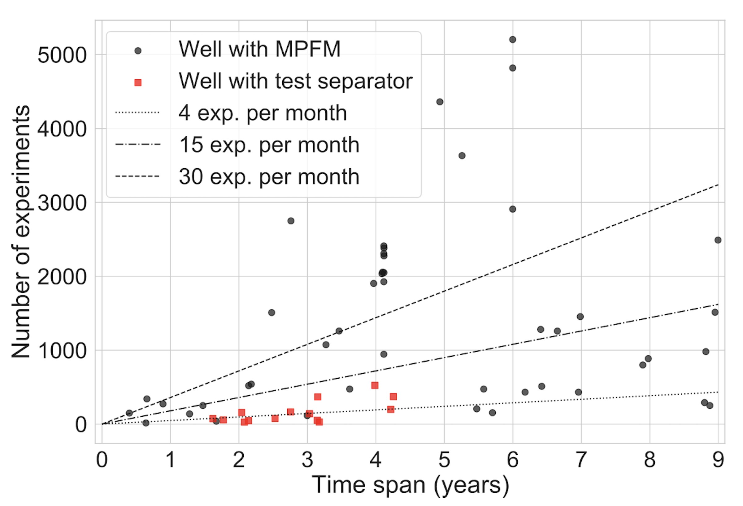
The dataset consists of 66367 experiments from 60 wells producing from five oil and gas fields. Figures 1 and 2 visualize the diverse characteristics of the dataset. For each well, we have a sequence of experiments in time. The time span from the first to the last experiment is plotted along the X-axis in Figure 1. The figure also shows that the experiment frequency varies from a handful to hundreds of experiments per year, as seen along the Y-axis of the same figure.

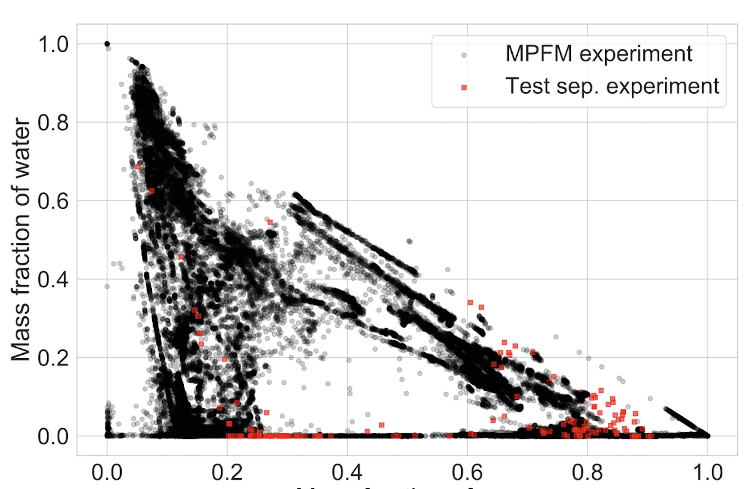
Each experiment consists of a measured total volumetric flow rate, either from a test separator, or a multiphase flow meter (MPFM), and measurements of the following explanatory variables: pressures and temperatures upstream and downstream the choke valve, choke opening, and mass fractions of oil and gas. 14 wells are tested with a test separator with an average of 163 experiments per well. The remaining 46 wells are tested with MPFMs with an average of 1393 experiments per well. The 60 wells are also quite different in terms of produced fluids, as illustrated in Figure 2.

Model estimation and architecture

The mean flow rates were modeled using feed-forward neural networks. The network architectures were fixed to three hidden layers, each with 50 nodes, to which we applied the ReLU activation function. The Adam optimizer was used to train the networks and we used early stopping with a validation dataset to avoid overfitting.

Non-stationarity is evident when comparing historical and future predictive results.

In our previous post about the main challenges of data-driven VFM modeling, we briefly touched upon the concern of having a non-stationary underlying process. This means that the distribution of values seen during training is not necessarily the same as the distribution of values used for testing.

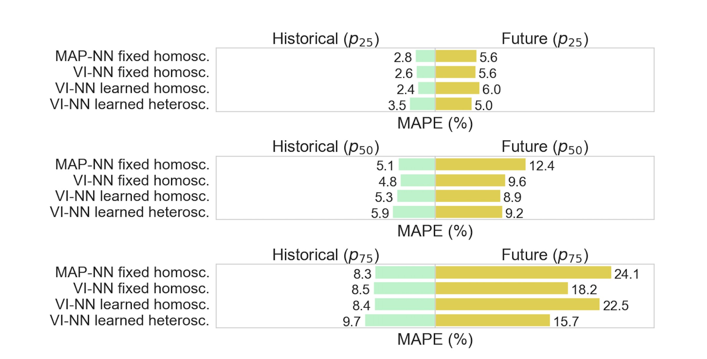
The non-stationarity effect is clearly observable in Figure 3 where we compare the predictive performance results of historical (green) versus future (yellow) data. This figure gives the mean absolute percentage error (MAPE) results across all wells. The test data comprises three months of chronological data, located in the middle of the dataset for historical performance analyses, and at the very end of the dataset for future performance analyses.

Looking at Figure 3, it is clear that the prediction error is consistently larger on future data than on historical data. Particularly, the MAPE of the 75% best performing future models is in the range of 16-24%, compared to 8-10% on historical data. Since the strength of data-driven models lies with interpolation, rather than extrapolation, it is natural that the performance is worse in the future data case. On the future data, the MAPE is around 9-13% or less for about half of the models. In our opinion, this is not robust enough for use in commercial VFM applications.

More sophisticated models have limited impact. Interestingly, all of the four model categories obtain comparable results on historical data. This means that neither more sophisticated noise models nor estimating the parameters with variational inference has a significant impact on the mean prediction value. In other words, this added complexity does not seem to pay off significantly for historical data. On future data, the VI-NN model with learned heteroscedastic noise seems to consistently outperform the MAP-NN models.

The variation in performance across wells is large.

0%

best case error [0.3%]

72%

worst case error [72.1%]

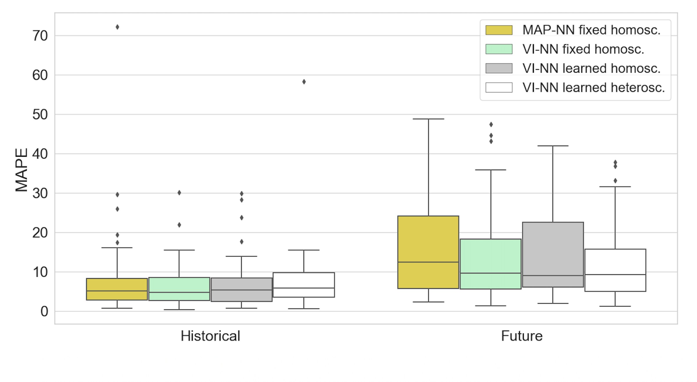
In the literature, errors of 10% or less are often cited in historical studies where NNs are used to model VFMs. In Figure 3 we can see that all four of our model categories are in line with these results on historical data, as they achieved a MAPE of <10% in 75% of the models. But to illustrate the high variation in performance, we include a boxplot of the results in Figure 4. It is illustrative to note that the overall best performing model achieved an error of 0.3%. The overall worst performing model achieved an error of 72.1%. This large variation makes us question the robustness of the approach.

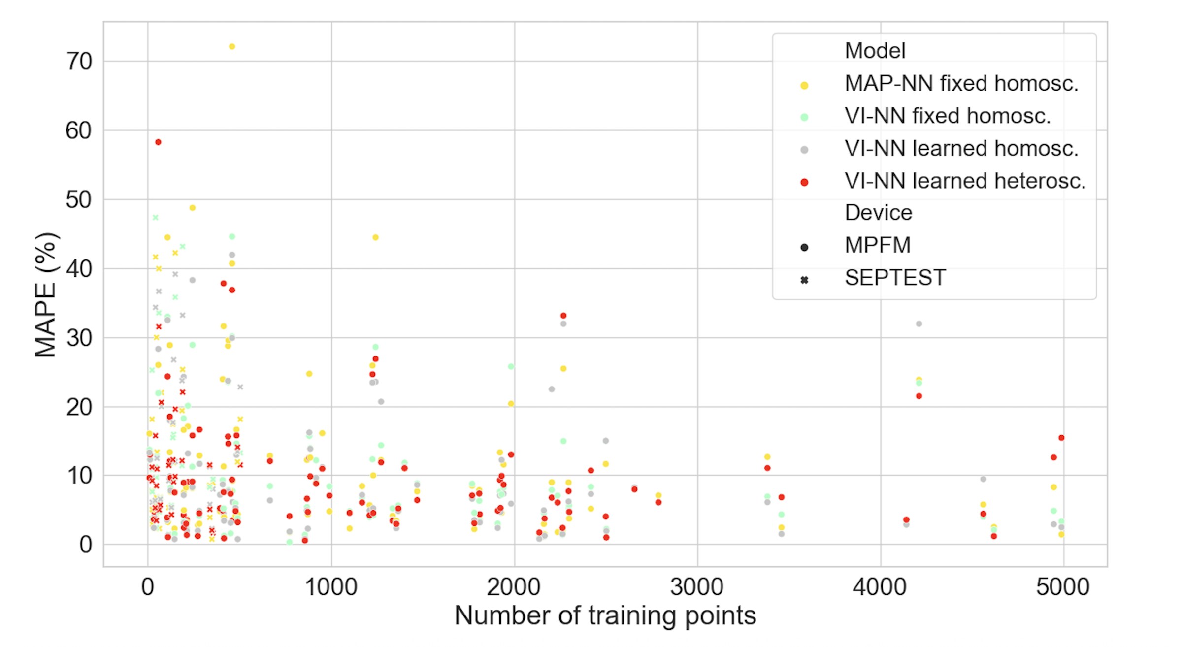
Data quantity outweighs data quality in the small-data regime

A closer look at the relationship between the MAPE obtained and the number of underlying data points in each individual well model, revealed that the variance in performance is higher among wells with less than 700 data points. This effect can be seen in Figure 5. This is concerning, because many of the wells in our study have fewer than 700 experiments to learn from, a situation that is probably quite common for most wells in operation. Somewhat surprisingly, we found that wells trained on MPFM data outperformed models trained on test separator data. The latter is considered high quality, but low quantity. This might indicate that data quantity outweighs data quality in the small data-regime that we are operating in.

What's next?

Stay tuned for our next posts, where we will dig into calibration plots in order to discuss prediction uncertainty provided by the variational inference estimation method. Prediction uncertainty is an important but often overlooked part of data-driven VFMs.

References

M. A. Ahmadi, M. Ebadi, A. Shokrollahi, S. M. J. Majidi, Evolving artificial neural network and imperialist competitive algorithm for prediction oil flow rate of the reservoir, Applied Soft Computing 13 (2013) 1085–1098.
T. A. AL-Qutami, R. Ibrahim, I. Ismail, M. A. Ishak, Radial basis function network to predict gas flow rate in multiphase flow., in: Proceedings of the 9th International Conference on Machine Learning and Computing, 2017,pp. 141–146.
T. A. AL-Qutami, R. Ibrahim, I. Ismail, M. A. Ishak, Development of soft sensor to estimate multiphase flow rates using neural networks and early stopping, in: International Journal on Smart Sensing and IntelligentSystems, Vol. 10, 2017, pp. 199–222
T. A. AL-Qutami, R. Ibrahim, I. Ismail, M. A. Ishak, Hybrid neural network and regression tree ensemble pruned by simulated annealing for virtual flow metering application, in: IEEE International Conference on Signal andImage Processing Applications (ICSIPA), 2017, pp. 304–309.
T. A. AL-Qutami, R. Ibrahim, I. Ismail, Virtual multiphase flow metering using diverse neural network ensemble and adaptive simulated annealing,Expert Systems With Applications 93 (2018) 72–85
S. M. Berneti, M. Shahbazian, An imperialist competitive algorithm - artificial neural network method to predict oil flow rate of the wells, International Journal of Computer Applications 26 (2011) 47–50
T. Bikmukhametov, J. Jäschke, Oil Production Monitoring Using GradientBoosting Machine Learning Algorithm, IFAC-PapersOnLine 52
M. Z. Hasanvand, S. Berneti, Predicting oil flow rate due to multiphase flow meter by using an artificial neural network, Energy Sources Part A Recovery Utilization and Environmental Effects 37 (2015) 840–845
Grimstad, B., Hotvedt, M., Sandnes, A.T., Kolbjørnsen, O., Imsland, L.S., 2021. Bayesian neural networks for virtual flow metering: An empirical study. arXiv:2102.01391